A simple self-attention mechanism
When an input is very long the RNNs fail because they cannot know the weight of each word in the sentence, for example in a long sentence maybe the words at the beginning have to do with the end but the RNNs do not know this. That is why we use attentional mechanisms that allow the model to know each weight of a token related to the rest of the input.
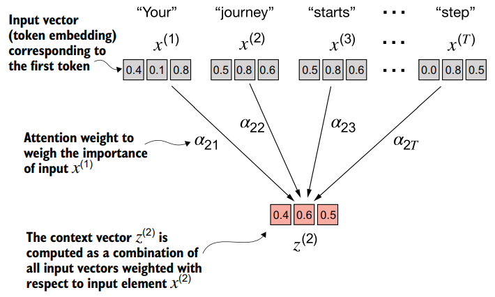 In self-attention, our goal is to calculate context vectors for each element in the input sequence. A context vector can be interpreted as an enriched embedding vector.
Calculate the scores
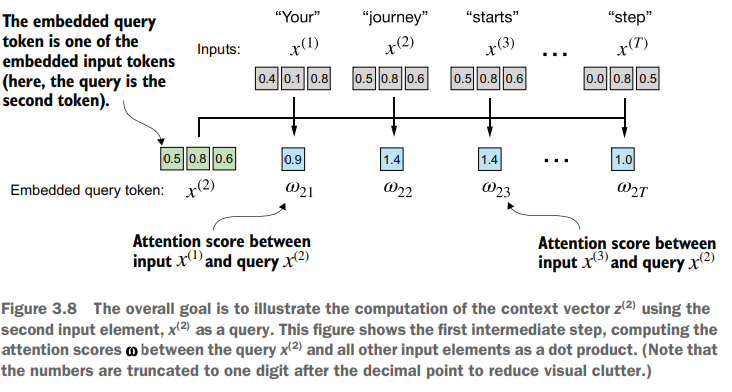
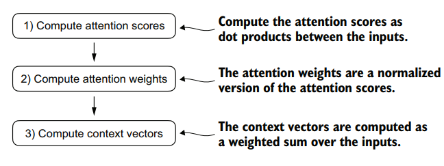
The first step is calculate the intermediate attention scores between the query token and each input token. We determine these scores by computing the dot product of the query, , with every other input token.
For calculate the scores we need to get the dot products of the vector with the each of the others.
For example, we want to get the attn_scores of the vector 2 in the following tensor:
inputs = torch.tensor(
    [
        [0.43, 0.15, 0.89],  # Your (x^1)
        [0.55, 0.87, 0.66],  # journey (x^2)
        [0.57, 0.85, 0.64],  # starts (x^3)
        [0.22, 0.58, 0.33],  # with (x^4)
        [0.77, 0.25, 0.10],  # one (x^5)
        [0.05, 0.80, 0.55],  # step (x^6)
    ]
)
We do a for loop for get the dot product of the [0.55, 0.87, 0.66] with the other vectors
query = inputs.shape[0]
atten_scores_2 = torch.empty(inputs.shape[0])

for i, x_i in enumerate(inputs):
    atten_scores_2[i] = torch.dot(x_i, query)

print(atten_scores_2)
What I do here is create a empty tensor with the shape of the input (totals rows 6) and then calculate each dot product related to query that is [0.55, 0.87, 0.66]
tensor([0.9544, 1.4950, 1.4754, 0.8434, 0.7070, 1.0865])Calculate the Attention Weights
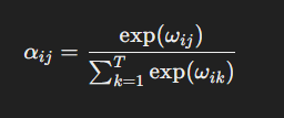
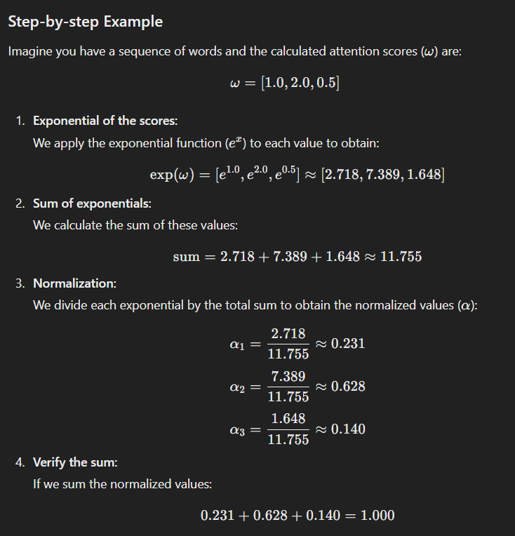
For calculate the attention weights normalize to 1 each element in atten_scores_2 this means that the sum of element in atten_scores_2 result to 1.
attn_weights_2_tmp = atten_scores_2 / atten_scores_2.sum()

print(atten_scores_2.sum())
print("Attention weights:", attn_weights_2_tmp)
print("Sum:", attn_weights_2_tmp.sum())tensor(6.5617)
Attention weights: tensor([0.1455, 0.2278, 0.2249, 0.1285, 0.1077, 0.1656]) Sum: tensor(1.0000)instead of that we can use the torch.sofmax() function
attn_weights_2 = torch.softmax(atten_scores_2, dim=0)

print("Attention weights:", attn_weights_2)
print("Sum:", attn_weights_2.sum())
Attention weights: tensor([0.1385, 0.2379, 0.2333, 0.1240, 0.1082, 0.1581])
Sum: tensor(1.)Calculating the context vector
We need to multiplying the embedded input tokens, with the corresponding attention weights and then summing the resulting vectors.
query = inputs[1]
context_vec_2 = torch.zeros(query.shape)
print(context_vec_2)
# print(attn_weights_2[4] * inputs[4] + attn_weights_2[3] * inputs[3])
for i, x_i in enumerate(inputs):
    context_vec_2 += attn_weights_2[i] * x_i

print(context_vec_2)
tensor([0., 0., 0.])
tensor([0.4419, 0.6515, 0.5683])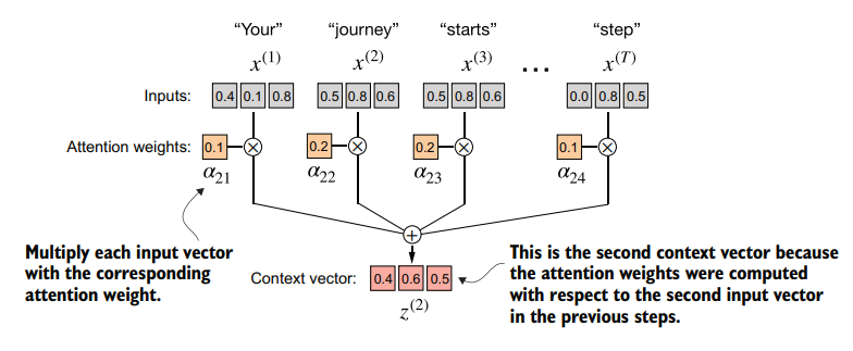
Computing attention weights for all input tokens
# Computing attention weights for all input tokens
attn_scores = torch.empty(6, 6)

# Compute attention scores
for i, x_i in enumerate(inputs):
    for j, x_j in enumerate(inputs):
        attn_scores[i, j] = torch.dot(x_i, x_j)

print(attn_scores)
tensor([[0.9995, 0.9544, 0.9422, 0.4753, 0.4576, 0.6310],
[0.9544, 1.4950, 1.4754, 0.8434, 0.7070, 1.0865],
[0.9422, 1.4754, 1.4570, 0.8296, 0.7154, 1.0605],
[0.4753, 0.8434, 0.8296, 0.4937, 0.3474, 0.6565],
[0.4576, 0.7070, 0.7154, 0.3474, 0.6654, 0.2935],
[0.6310, 1.0865, 1.0605, 0.6565, 0.2935, 0.9450]])Get the same result doing:
# matrix multiplication
attn_scores = inputs @ inputs.T
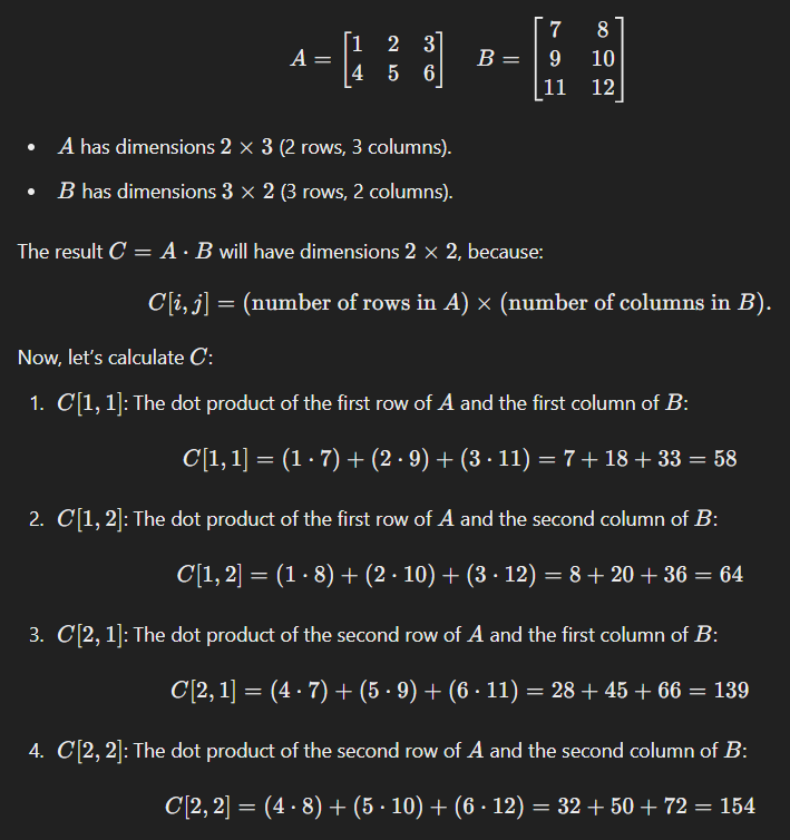
print(attn_scores)Rules for multiplying matrices
To multiply two matrices, say 𝐴 and 𝐵, they must meet the following condition:
- The number of columns of A must be equal to the number of rows of B.
- If 𝐴 has the shape (𝑚×𝑛) y 𝐵 has the shape (𝑛×𝑝), then the product 𝐶=𝐴⋅𝐵 will have the shape (𝑚×𝑝).
# Compute attention weights
attn_weights = torch.softmax(attn_scores, dim=-1)
print(attn_weights)
tensor([[0.2098, 0.2006, 0.1981, 0.1242, 0.1220, 0.1452],
[0.1385, 0.2379, 0.2333, 0.1240, 0.1082, 0.1581],
[0.1390, 0.2369, 0.2326, 0.1242, 0.1108, 0.1565],
[0.1435, 0.2074, 0.2046, 0.1462, 0.1263, 0.1720],
[0.1526, 0.1958, 0.1975, 0.1367, 0.1879, 0.1295],
[0.1385, 0.2184, 0.2128, 0.1420, 0.0988, 0.1896]])# Compute context vectors
all_context_vecs = attn_weights @ inputs
print(all_context_vecs)tensor([[0.4421, 0.5931, 0.5790],
[0.4419, 0.6515, 0.5683],
[0.4431, 0.6496, 0.5671],
[0.4304, 0.6298, 0.5510],
[0.4671, 0.5910, 0.5266],
[0.4177, 0.6503, 0.5645]])Implementing self-attention with trainable weights
The most popular GPTs models use self-attention mechanism called scaled dot-product attention.
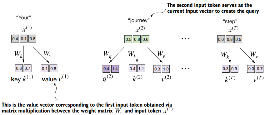
This mechanism introduce weight matrices that are updated during model training. These trainable weight matrices are crucial so that the model (specifically, the attention module inside the model) can learn to produce “good” context vectors.
Computing the attention weights
These matrices are used to project the input token into query, key and value vectors.
class SelfAttention_v1(nn.Module):
    def __init__(self, d_in, d_out):
        super().__init__()
        self.W_query = nn.Parameter(torch.rand(d_in, d_out))
        self.W_key = nn.Parameter(torch.rand(d_in, d_out))
        self.W_value = nn.Parameter(torch.rand(d_in, d_out))

    def forward(self, x):
        keys = x @ self.W_key
        queries = x @ self.W_query
        values = x @ self.W_value
        attn_scores = queries @ keys.T  # omega
        attn_weights = torch.softmax(attn_scores / keys.shape[-1] ** 0.5, dim=-1)
        context_vec = attn_weights @ values
return context_vec- Input parameters:
d_in: The dimensionality of the input embeddings.d_out: The dimensionality of the output embeddings.
- Weight matrices: -
W_query,W_key, andW_valueare learnable parameters initialized randomly. These matrices transform the input into query, key, and value vectors. - Theforwardmethod defines how the input tensorxflows through the model.
The input x (shape [batch_size, d_in]) is projected into:
- Keys:
x @ W_key(shape[batch_size, d_out]) - Queries:
x @ W_query(shape[batch_size, d_out]) - Values:
x @ W_value(shape[batch_size, d_out])
torch.manual_seed(123)

sa_v1 = SelfAttention_v1(d_in, d_out)
print(sa_v1(inputs))
tensor([[0.2996, 0.8053],
[0.3061, 0.8210],
[0.3058, 0.8203],
[0.2948, 0.7939],
[0.2927, 0.7891],
[0.2990, 0.8040]], grad_fn=<MmBackward0>)A self-attention class using PyTorch’s Linear layers
class SelfAttention_v2(nn.Module):
def __init__(self, d_in, d_out, qkv_bias=False):
super().__init__()
self.W_query = nn.Linear(d_in, d_out, bias=qkv_bias)
self.W_key = nn.Linear(d_in, d_out, bias=qkv_bias)
self.W_value = nn.Linear(d_in, d_out, bias=qkv_bias)
def forward(self, x):
keys = self.W_key(x)
queries = self.W_query(x)
values = self.W_value(x)
attn_scores = queries @ keys.T
attn_weights = torch.softmax(attn_scores / keys.shape[-1] ** 0.5, dim=-1)
context_vec = attn_weights @ values
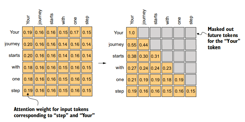
return context_vecCausal attention AKA masked attention
It restricts a model to only consider previous and current inputs in sequence when processing any given token when computing attention scores.
for each token processed, we mask out the future tokens, which come after the current token in the input text.
torch.manual_seed(789)
sa_v2 = SelfAttention_v2(d_in, d_out)

queries = sa_v2.W_query(inputs)
keys = sa_v2.W_key(inputs)
attn_scores = queries @ keys.T
attn_weights = torch.softmax(attn_scores / keys.shape[-1]**0.5, dim=-1)

print(attn_weights)
tensor([[0.1921, 0.1646, 0.1652, 0.1550, 0.1721, 0.1510],
[0.2041, 0.1659, 0.1662, 0.1496, 0.1665, 0.1477],
[0.2036, 0.1659, 0.1662, 0.1498, 0.1664, 0.1480],
[0.1869, 0.1667, 0.1668, 0.1571, 0.1661, 0.1564],
[0.1830, 0.1669, 0.1670, 0.1588, 0.1658, 0.1585],
[0.1935, 0.1663, 0.1666, 0.1542, 0.1666, 0.1529]],
grad_fn=<SoftmaxBackward0>)Implementing a simple mask
context_length = attn_scores.shape[0]
mask_simple = torch.tril(torch.ones(context_length, context_length))
print(mask_simple)
tensor([[1., 0., 0., 0., 0., 0.],
[1., 1., 0., 0., 0., 0.],
[1., 1., 1., 0., 0., 0.],
[1., 1., 1., 1., 0., 0.],
[1., 1., 1., 1., 1., 0.],
[1., 1., 1., 1., 1., 1.]])multiply this mask with the attention weights to zero-out the values above the diagonal:
masked_simple = attn_weights*mask_simple
print(masked_simple)
tensor([[0.1921, 0.0000, 0.0000, 0.0000, 0.0000, 0.0000],
[0.2041, 0.1659, 0.0000, 0.0000, 0.0000, 0.0000],
[0.2036, 0.1659, 0.1662, 0.0000, 0.0000, 0.0000],
[0.1869, 0.1667, 0.1668, 0.1571, 0.0000, 0.0000],
[0.1830, 0.1669, 0.1670, 0.1588, 0.1658, 0.0000],
[0.1935, 0.1663, 0.1666, 0.1542, 0.1666, 0.1529]],
grad_fn=<MulBackward0>)renormalize the attention weights to sum up to 1
row_sums = masked_simple.sum(dim=-1, keepdim=True)
masked_simple_norm = masked_simple / row_sums
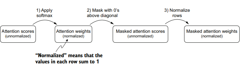
print(masked_simple_norm)The softmax function takes a vector of values and converts them into a probability distribution. The formula is:
1. Very negative values :
- , which completely removes the contribution of that position to the attention calculation. This means the masked position will have exactly 000 probability.
2. Zero values (000):
- , meaning the masked position still contributes to the denominator. This can lead to an incorrect probability distribution because positions that should be ignored are still being considered.
The softmax function converts its inputs into a probability distribution. When negative infinity values are present in a row, the softmax function treats them as zero probability. (Mathematically, this is because approaches 0.) We can implement this more efficient masking “trick” by creating a mask with 1s above the diagonal and then replacing these 1s with negative infinity (-inf) values:
mask = torch.triu(torch.ones(context_length, context_length), diagonal=1)
masked = attn_scores.masked_fill(mask.bool(), -torch.inf)
print(masked)
tensor([[0.2899, -inf, -inf, -inf, -inf, -inf],
[0.4656, 0.1723, -inf, -inf, -inf, -inf],
[0.4594, 0.1703, 0.1731, -inf, -inf, -inf],
[0.2642, 0.1024, 0.1036, 0.0186, -inf, -inf],
[0.2183, 0.0874, 0.0882, 0.0177, 0.0786, -inf],
[0.3408, 0.1270, 0.1290, 0.0198, 0.1290, 0.0078]],
grad_fn=<MaskedFillBackward0>)attn_weights = torch.softmax(masked / keys.shape[-1]**0.5, dim=1)
print(attn_weights)tensor([[1.0000, 0.0000, 0.0000, 0.0000, 0.0000, 0.0000],
[0.5517, 0.4483, 0.0000, 0.0000, 0.0000, 0.0000],
[0.3800, 0.3097, 0.3103, 0.0000, 0.0000, 0.0000],
[0.2758, 0.2460, 0.2462, 0.2319, 0.0000, 0.0000],
[0.2175, 0.1983, 0.1984, 0.1888, 0.1971, 0.0000],
[0.1935, 0.1663, 0.1666, 0.1542, 0.1666, 0.1529]],
grad_fn=<SoftmaxBackward0>)context_vec = attn_weights @ values
print(context_vec)tensor([[0.1855, 0.8812],
[0.2795, 0.9361],
[0.3133, 0.9508],
[0.2994, 0.8595],
[0.2702, 0.7554],
[0.2772, 0.7618]], grad_fn=<MmBackward0>)Masking additional attention weights with dropout
Dropout in deep learning is a technique where randomly selected hidden layer units are ignored during training, effectively “dropping” them out. This method helps prevent overfitting by ensuring that a model does not become overly reliant on any specific set of hidden layer units. It’s important to emphasize that dropout is only used during training and is disabled afterward.
torch.manual_seed(123)
dropout = torch.nn.Dropout(0.5) # We choose a dropout rate of 50%.
example = torch.ones(6, 6) # Here, we create a matrix of 1s.
print(dropout(example))
tensor([[2., 2., 2., 2., 2., 2.],
[0., 2., 0., 0., 0., 0.],
[0., 0., 2., 0., 2., 0.],
[2., 2., 0., 0., 0., 2.],
[2., 0., 0., 0., 0., 2.],
[0., 2., 0., 0., 0., 0.]])apply dropout to the attention weight matrix itself:
torch.manual_seed(123)
print(dropout(attn_weights))
tensor([[2.0000, 0.0000, 0.0000, 0.0000, 0.0000, 0.0000],
[0.0000, 0.8966, 0.0000, 0.0000, 0.0000, 0.0000],
[0.0000, 0.0000, 0.6206, 0.0000, 0.0000, 0.0000],
[0.5517, 0.4921, 0.0000, 0.0000, 0.0000, 0.0000],
[0.4350, 0.0000, 0.0000, 0.0000, 0.0000, 0.0000],
[0.0000, 0.3327, 0.0000, 0.0000, 0.0000, 0.0000]],
grad_fn=<MulBackward0>)Implementing a compact causal attention class
We will now incorporate the causal attention and dropout modifications into the SelfAttention Python class.
# Two inputs with six tokens each; each token has embedding dimension 3.
batch = torch.stack((inputs, inputs), dim=0)
print(batch.shape)
This results in a three-dimensional tensor consisting of two input texts with six tokens each, where each token is a three-dimensional embedding vector:
torch.Size([2, 6, 3])Casual Attention Class:
class CausalAttention(nn.Module):
    def __init__(self, d_in, d_out, context_length, dropout, qkv_bias=False):
        super().__init__()
        self.d_out = d_out
        self.W_query = nn.Linear(d_in, d_out, bias=qkv_bias)
        self.W_key = nn.Linear(d_in, d_out, bias=qkv_bias)
        self.W_value = nn.Linear(d_in, d_out, bias=qkv_bias)
        self.dropout = nn.Dropout(dropout) # added a dropout layer.
        self.register_buffer(
            "mask", torch.triu(torch.ones(context_length, context_length), diagonal=1)
        )

    def forward(self, x):
        b, num_tokens, d_in = x.shape
        keys = self.W_key(x)
        queries = self.W_query(x)
        values = self.W_value(x)
        # transpose dimensions 1 and 2, keeping the batch
        # dimension at the first position (0).
        attn_scores = queries @ keys.transpose(1, 2)
        attn_scores.masked_fill_(self.mask.bool()[:num_tokens, :num_tokens], -torch.inf)
        attn_weights = torch.softmax(attn_scores / keys.shape[-1] ** 0.5, dim=-1)
        attn_weights = self.dropout(attn_weights)
        context_vec = attn_weights @ values
return context_vectorch.manual_seed(123)
context_length = batch.shape[1]
ca = CausalAttention(d_in, d_out, context_length, 0.0)
context_vecs = ca(batch)
print("context_vecs.shape:", context_vecs.shape)The resulting context vector is a three-dimensional tensor where each token is now represented by a two-dimensional embedding:
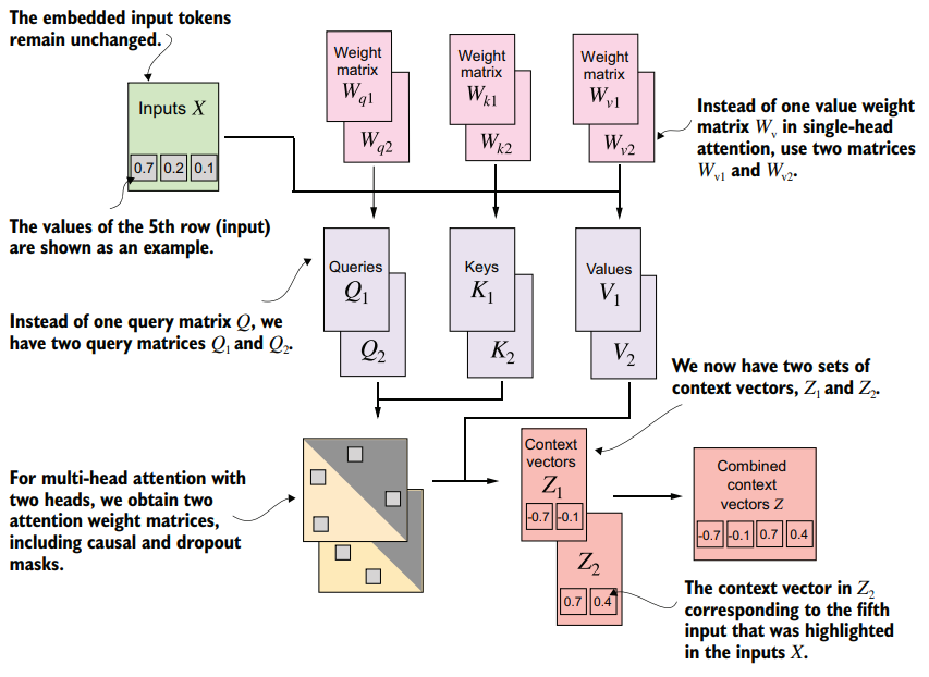
context_vecs.shape: torch.Size([2, 6, 2])Multi-head attention
The main idea behind multi-head attention is to run the attention mechanism multiple times (in parallel) with different, learned linear projections—the results of multiplying the input data (like the query, key, and value vectors in attention mechanisms) by a weight matrix.
“multi-head” refers to dividing the attention mechanism into multiple “heads,” each operating independently.
class MultiHeadAttentionWrapper(nn.Module):
    def __init__(self, d_in, d_out, context_length, dropout, num_heads, qkv_bias=False):
        super().__init__()
        self.heads = nn.ModuleList(
            [
                CausalAttention(d_in, d_out, context_length, dropout, qkv_bias)
                for _ in range(num_heads)
            ]
        )

    def forward(self, x):
return torch.cat([head(x) for head in self.heads], dim=-1)torch.manual_seed(123)
context_length = batch.shape[1] # This is the number of tokens
d_in, d_out = 3, 2
mha = MultiHeadAttentionWrapper(d_in, d_out, context_length, 0.0, num_heads=2)
context_vecs = mha(batch)
print(context_vecs)
print("context_vecs.shape:", context_vecs.shape)This results in the following tensor representing the context vectors:
tensor([[[-0.4519, 0.2216, 0.4772, 0.1063],
		[-0.5874, 0.0058, 0.5891, 0.3257],
		[-0.6300, -0.0632, 0.6202, 0.3860],
		[-0.5675, -0.0843, 0.5478, 0.3589],
		[-0.5526, -0.0981, 0.5321, 0.3428],
		[-0.5299, -0.1081, 0.5077, 0.3493]],

		[[-0.4519, 0.2216, 0.4772, 0.1063],
		[-0.5874, 0.0058, 0.5891, 0.3257],
		[-0.6300, -0.0632, 0.6202, 0.3860],
		[-0.5675, -0.0843, 0.5478, 0.3589],
		[-0.5526, -0.0981, 0.5321, 0.3428],
		[-0.5299, -0.1081, 0.5077, 0.3493]]], grad_fn=<CatBackward0>)
context_vecs.shape: torch.Size([2, 6, 4])
Implementing multi-head attention with weight splits
On a big-picture level, in the previous MultiHeadAttentionWrapper, we stacked
multiple single-head attention layers that we combined into a multi-head attention
layer. The MultiHeadAttention class takes an integrated approach. It starts with a
multi-head layer and then internally splits this layer into individual attention heads.
The splitting of the query, key, and value tensors is achieved through tensor reshaping and transposing operations using PyTorch’s .view and .transpose methods. The
input is first transformed (via linear layers for queries, keys, and values) and then
reshaped to represent multiple heads.
class MultiHeadAttention(nn.Module):
    def __init__(self, d_in, d_out, context_length, dropout, num_heads, qkv_bias=False):
        super().__init__()
        assert d_out % num_heads == 0, "d_out must be divisible by num_heads"
        self.d_out = d_out
        self.num_heads = num_heads
        self.head_dim = d_out // num_heads
        self.W_query = nn.Linear(d_in, d_out, bias=qkv_bias)
        self.W_key = nn.Linear(d_in, d_out, bias=qkv_bias)
        self.W_value = nn.Linear(d_in, d_out, bias=qkv_bias)
        self.out_proj = nn.Linear(d_out, d_out)
        self.dropout = nn.Dropout(dropout)
        self.register_buffer(
            "mask", torch.triu(torch.ones(context_length, context_length), diagonal=1)

        )

    def forward(self, x):
        b, num_tokens, d_in = x.shape
        keys = self.W_key(x)
        queries = self.W_query(x)
        values = self.W_value(x)

        keys = keys.view(b, num_tokens, self.num_heads, self.head_dim)
        values = values.view(b, num_tokens, self.num_heads, self.head_dim)
        queries = queries.view(b, num_tokens, self.num_heads, self.head_dim)
        # Transposes from shape (b, num_tokens, num_heads, head_dim)
        # to (b, num_heads, num_tokens, head_dim)
        keys = keys.transpose(1, 2)
        queries = queries.transpose(1, 2)
        values = values.transpose(1, 2)

        attn_scores = queries @ keys.transpose(2, 3)
        mask_bool = self.mask.bool()[:num_tokens, :num_tokens]

        attn_scores.masked_fill_(mask_bool, -torch.inf)

        attn_weights = torch.softmax(attn_scores / keys.shape[-1] ** 0.5, dim=-1)
        attn_weights = self.dropout(attn_weights)

        context_vec = (attn_weights @ values).transpose(1, 2)

        context_vec = context_vec.contiguous().view(b, num_tokens, self.d_out)
        context_vec = self.out_proj(context_vec)
        return context_vec
The tensors are then transposed to bring the num_heads dimension before the num_ tokens dimension, resulting in a shape of (b, num_heads, num_tokens, head_dim). This transposition is crucial for correctly aligning the queries, keys, and values across the different heads and performing batched matrix multiplications efficiently. To illustrate this batched matrix multiplication, suppose we have the following tensor:
# The shape of this tensor is
# (b, num_heads, num_tokens, head_dim) = (1, 2, 3, 4).
a = torch.tensor(
    [
        [
            [
                [0.2745, 0.6584, 0.2775, 0.8573],
                [0.8993, 0.0390, 0.9268, 0.7388],
                [0.7179, 0.7058, 0.9156, 0.4340],
            ],
            [
                [0.0772, 0.3565, 0.1479, 0.5331],
                [0.4066, 0.2318, 0.4545, 0.9737],
                [0.4606, 0.5159, 0.4220, 0.5786],
            ],
        ]
    ]
)

print(a @ a.transpose(2, 3))

first_head = a[0, 0, :, :]
first_res = first_head @ first_head.T
print("First head:\n", first_res)
second_head = a[0, 1, :, :]
second_res = second_head @ second_head.T
print("\nSecond head:\n", second_res)
tensor([[[[1.3208, 1.1631, 1.2879],
[1.1631, 2.2150, 1.8424],
[1.2879, 1.8424, 2.0402]],
[[0.4391, 0.7003, 0.5903],
[0.7003, 1.3737, 1.0620],
[0.5903, 1.0620, 0.9912]]]])
First head:
tensor([[1.3208, 1.1631, 1.2879],
[1.1631, 2.2150, 1.8424],
[1.2879, 1.8424, 2.0402]])
Second head:
tensor([[0.4391, 0.7003, 0.5903],
[0.7003, 1.3737, 1.0620],
[0.5903, 1.0620, 0.9912]])torch.manual_seed(123)
batch_size, context_length, d_in = batch.shape
d_out = 2
mha = MultiHeadAttention(d_in, d_out, context_length, 0.0, num_heads=2)
context_vecs = mha(batch)
print(context_vecs)
print("context_vecs.shape:", context_vecs.shape)tensor([[[0.3190, 0.4858],
[0.2943, 0.3897],
[0.2856, 0.3593],
[0.2693, 0.3873],
[0.2639, 0.3928],
[0.2575, 0.4028]],
[[0.3190, 0.4858],
[0.2943, 0.3897],
[0.2856, 0.3593],
[0.2693, 0.3873],
[0.2639, 0.3928],
[0.2575, 0.4028]]], grad_fn=<ViewBackward0>)
context_vecs.shape: torch.Size([2, 6, 2])